Substructuring example: Benfield truss
The goal of this notebook is to summarize and benchmark the methodology applied and learnt during the IMAC shortcourse titled Short Course on Experimental Dynamic Substructuring, during the 2020 conference.
Outline of methodology
Some of the most important details about the substructuring methodology is provided below; please refer to the slides or the cited literature for more details.

The following three equations describe the full problem:
- The system can be described by the following equation of motion including coupling forces $\{g\}$:
The system matrices and force/response vectors above are established by stacking the contributions from all $n$ substructures as exemplified with the stiffness matrix and the displacement vector here:
$$ [K] = \begin{bmatrix} [K]^{(1)} & & & \\ & [K]^{(2)} & & \\ & & \ddots & \\ & & & [K]^{(n)} \end{bmatrix}, \qquad \{u\} = \begin{Bmatrix} \{u\}^{(1)} \\ \{u\}^{(2)} \\ \vdots \\\{u\}^{(n)} \end{Bmatrix}$$- We require compatiblity at the interfaces (displacements are equal of matching nodes):
- The interface forces are in equilibrium (actio-reactio): $$[L]^T\{g\} = \{0\}$$
$[L]$ and $[B]$ are typically boolean matrices (contain only 1 and 0), and are related as follows:
$$[B][L] = [0] \quad \Rightarrow \quad [L] = \text{null }[B]$$Two approaches (presented in the two following subsections) to assemble the substructures were presented in the course:
- Primal assembly, which is based on removing rows and columns of the matrices (and corresponding rows from the vectors). This can be achieved by utilizing $[L]$.
- Dual assembly, which is based on adding Lagrange multiplier constraints tieing DOFs together. This can be achieved by utilizing $[B]$.
Primal assembly
The assembled problem is rewritten with only compatible DOFs, i.e., only keeping one unique DOF for each interface constraint. Formally, this can be expressed through the subset of the DOFs $\{u\}$, denoted $\{\tilde{u}$} (or as $\{u_{glob}\}$ in course slides), which is defined through the following relation:
$$ \{u\} = [L] \{\tilde{u}\} $$Then, the equation of motion is rewritten as:
$$[M][L] \{\ddot{\tilde{u}}\} + [C] [L] \{\dot{\tilde{u}}\} + [K][L] \{\tilde{u}\} = \{f\} + \{g\}$$By premultiplication with $[L]^T$ we can utlize the fact that $[L]^T\{g\}=\{0\}$, and thus get rid of the connection forces as follows:
$$[L]^T[M][L] \{\ddot{\tilde{u}}\} +[L]^T [C] [L] \{\dot{\tilde{u}}\} + [L]^T[K][L] \{\tilde{u}\} = [L]^T\{f\}$$Thus, the new system matrices and vectors are related to the original through the following relations: $$[\tilde{M}] = [L]^T[M][L]$$ $$[\tilde{C}] = [L]^T[C][L]$$ $$[\tilde{K}] = [L]^T[K][L]$$ $$\{\tilde{f}\} = [L]^T \{f\}$$ $$ \{u\} = [L] \{\tilde{u}\} $$
Dual assembly
Now, we define the coupling forces as follows:
$$ \{g\} = -[B]^T \{\lambda\}$$where $\{\lambda\}$ is a set of Lagrange multipliers, ensuring that $\{g\}$ provide equilibrium at the interface.
Combining this with $[B]\{u\} = \{0\}$ and the original equation of motion, the following new equation of motion can be established:
$$ \begin{bmatrix} [M] & [0] \\ [0] & [0] \end{bmatrix} \begin{Bmatrix}\{\ddot{u}\} \\ \{\lambda\} \end{Bmatrix}+ \begin{bmatrix} [C] & [0] \\ [0] & [0] \end{bmatrix} \begin{Bmatrix}\{\dot{u}\} \\ \{\lambda\} \end{Bmatrix}+ \begin{bmatrix} [K] & [B]^T \\ [B] & [0] \end{bmatrix} \begin{Bmatrix}\{u\} \\ \{\lambda\} \end{Bmatrix} = \begin{Bmatrix} \{f\} \\ \{0\}\end{Bmatrix} $$Because the boundaries of an interface are not necessarily matching perfectly (either because substructures do not fit or because the substructures are separately represented by a limited number of modes, not guaranteeing a perfect compatibility), the ability to relax constraints makes the dual assembly a better choice in practical (and particularily, experimental) substructuring. Furthermore, all connection forces can be readily computed through $ \{g\} = -[B]^T \{\lambda\}$.
Dual assembly in modal space
First, the DOFs of a substructure is written as: $$ \{u\}^{(s)} \approx [R]^{(s)}\{\eta\}^{(s)}$$
Here, $[R]^{(s)}$ is introduced as the reduced set of mode shapes corresponding to substructure $s$, in contrast to $[\phi]^{(s)}$ which contains the full set of mode shapes for the same substructure (and does thus represent an exact representation). For all substructures combined, this can be accomplished by grouping the mode shapes in block-matrices as follows:
$$\{u\} \approx [R]\{\eta\}$$where $[R]= \begin{bmatrix} [R]^{(1)} & & & \\ & [R]^{(2)} & & \\ & & \ddots & \\ & & &[R]^{(n)}\end{bmatrix}$
The equation of motion can thus be approximated by the (truncated) modal space as follows: $$ [M_m]\{\ddot{\eta}\} + [C_m]\{\dot{\eta}\} + [K_m]\{\eta\} = \{f_m\} + \{g_m\}$$
where modal transformations are on the following form: $$[M_m]= [R]^T[M][R], \qquad \{f_m\} = [R]^T\{f\}$$
Also, the compatibility condition $[B]\{u\} = \{0\}$ is also transformed as follows:
$$[B_m] = [B][R], \qquad [B_m]\{\eta\}=\{0\}$$Thus, by following the example of the physical assembly, the modal substructures can be assembled in the following manner:
$$ \begin{bmatrix} [M_m] & [0] \\ [0] & [0] \end{bmatrix} \begin{Bmatrix}\{\ddot{\eta}\} \\ \{\lambda\} \end{Bmatrix}+ \begin{bmatrix} [C_m] & [0] \\ [0] & [0] \end{bmatrix} \begin{Bmatrix}\{\dot{\eta}\} \\ \{\lambda\} \end{Bmatrix}+ \begin{bmatrix} [K_m] & [B_m]^T \\ [B_m] & [0] \end{bmatrix} \begin{Bmatrix}\{\eta\} \\ \{\lambda\} \end{Bmatrix} = \begin{Bmatrix} \{f_m\} \\ \{0\}\end{Bmatrix} $$The subselection of modes in $[R]$ (from all substructures) is crucial for a proper representation of the combined response of the structure; for instance, rigid body modes should be included. Also, weakening of the interface is a necessity (not considered here).
System definition
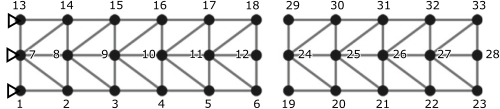
The Benfield truss from Benfield and Hruda (1971), and reproduced on page 40 in Allen et al. (2020), is used as example. The truss and the chosen node labeling used for this example is given below.
The following four tests are conducted:
- Dual assembly $\rightarrow$ static response prediction, serving as a qualitative compatibility check
- Primal assembly of the substructures $\rightarrow$ modal analysis of full system
- Dual assembly of the substructures $\rightarrow$ modal analysis of full system
- Dual assembly based on the complete modal representations of the substructures $\rightarrow$ modal analysis of the full system
The left and right parts are separated and defined as two substructures of the same structure. For the example herein, a 1-meter grid is assumed; e.g., the distance between node 1 and 2 or 1 and 7 are 1m. Note that the distance between the substructures is arbitrarily chosen, and as the DOFs of the interface nodes are defined equal, it is irrelevant.
The system is defined programatically through the node_matrix and element_matrix arrays. They are described below:
node_matrix: Each row defines a node; first column defines label, second label defines x-position, third label defines y-position.
Example row: [node_label,x,y]element_matrix: Each row defines an element; first column defines label, second column defines label of the first node, third column defines label of the second node.
Example row: [element_label,node_label_1,node_label_2].
The following code defines the system (note that the example_input module simply contains functions defining the element_matrix and node_matrix of the left and right part, as this is considered unimportant for the example):
# Loading required modules
import example_input
import febar as fe
import numpy as np
import matplotlib.pyplot as plt
from scipy.linalg import eig, block_diag, null_space as null
x0 = 6.0  # x-coordinate of the start of the rightmost substructure
phi_plot = dict() # empty dictionary to store plotting results
max_u_plot = 0.6      # max u to plot (scale largest displacement to this value)

# Retrieving node and element matrices
node_matrix_left, element_matrix_left = example_input.left_part()
node_matrix_right, element_matrix_right = example_input.right_part(x0=x0)

# Combining both substructures to common node_matrix and element_matrix
node_matrix = np.vstack([node_matrix_left, node_matrix_right])
element_matrix = np.vstack([element_matrix_left, element_matrix_right])

# Material properties
E = 210e9
A = 0.05
m = 1.0

# Define part object
part = fe.Part(node_matrix, element_matrix, E=E, A=A, m=m)

# Construct system matrices from part object
K = part.assemble(matrix_type='k')
M = part.assemble(matrix_type='m')
n_dofs = K.shape[0]
The system resulting from the defined nodes and elements can be plotted, as follows:
plt.figure(1)
plt.clf()

ax = part.plot(node_labels=True, element_labels=False)

ax.grid()
__ = ax.axis('equal')

Definition of connectivity / constraints
The constraints are defined through the array dof_pairs with a row for each constraint dof definition. The first column corresponds to the master degree of freedom (DOF) and the second column to the slave DOF. If the slave DOF is defined as None, it is assumed to be grounded.
The following nodes are assumed fully connected: 6$\leftrightarrow$19, 12$\leftrightarrow$24, 18$\leftrightarrow$29. Furthermore, the system is assumed fully grounded in nodes 1,7, and 13. The code to define this is given below.
# Defining constraint nodes
fixed_nodes = [1,7,13]         # ground-fixed
conn_nodes_left = [6,12,18]    # left substructure connections
conn_nodes_right = [19,24,29]  # right substructure connections

# Convert node labels to global DOF indices
fixed_dofs = part.gdof_ix_from_nodelabel(fixed_nodes)
conn_dofs_left = part.gdof_ix_from_nodelabel(conn_nodes_left)
conn_dofs_right = part.gdof_ix_from_nodelabel(conn_nodes_right)

# Construct 2d array with all constraint node definitions
dof_pairs = np.vstack(
                        [np.vstack([fixed_dofs, [None]*len(fixed_dofs)]).T,
                         np.vstack([conn_dofs_left,conn_dofs_right]).T]
    )

print(f'dof_pairs = \n\n {dof_pairs} \n')
For convenience, the function compatibility_matrix found inside the febar module used to establish $[B]$ is shown below:
def compatibility_matrix(dof_pairs, n_dofs):
    n_constraints = dof_pairs.shape[0]
    B = np.zeros([n_constraints, n_dofs])

    for constraint_ix, dof_pair in enumerate(dof_pairs):
        if dof_pair[1] is None:    # connected dof is None --> fixed to ground
            B[constraint_ix, dof_pair[0]] = 1
        else:
            B[constraint_ix, dof_pair[0]] = 1
            B[constraint_ix, dof_pair[1]] = -1
    return B
Test 1: Static response prediction
The stiffness matrix is constrained by introducing Lagrange multipliers as new constraint DOFs. The stiffness matrix can be constrained by enforcing motions as defined by $[B]$:
$[K_{lagr}]=\begin{bmatrix} [K] & [B]^T \\ [B] & [0] \end{bmatrix}$
This is implemented in the function lagrange_constrain:
K_lagr = fe.lagrange_constrain(K, dof_pairs)      # construct stiffness matrix, expanded with [B] and [B]^T to constrain
B = fe.compatibility_matrix(dof_pairs, n_dofs)    # B matrix
n_constr = dof_pairs.shape[0]                     # number of constraints
# Defining load in node 28, vertical (i.e., index 1)
f = np.zeros([n_dofs, 1])
dof_ix_load = part.gdof_ix_from_nodelabel(28, 1)
f[dof_ix_load] = -20e3

# Treatment of Lagrange DOFs and predict response
f_lagr = np.vstack([f, np.zeros([n_constr, 1])])   # expand f vector with zeros for constraint DOFs
u_lagr = np.linalg.inv(K_lagr) @ f_lagr            # predict response through K^-1 . f
g_constr = -B.T @ u_lagr[-n_constr:, :]            # obtain constraint forces
u = u_lagr[0:-n_constr, :]                         # subselect response values of physical DOFs
u_plot = u/np.max(abs(u))*max_u_plot

ax = part.plot(node_labels=False, element_labels=False, u=None)
part.plot(node_labels=False, element_labels=False, color='IndianRed', u=u_plot)
ax.grid()
__ = ax.axis('equal')

Well, that looks dandy!
Test 2: Primal assembly, modal analysis
In primal assembly, the mass and stiffness (and damping, in general) matrices are modified such that rows and columns corresponding to fixed DOFs are removed whereas rows and columns of the connected DOFs are combined. This can be established by utilizing the $[L]$ matrix as follows:
$$[\tilde{M}] = [L]^T[M][L]$$$$[\tilde{K}] = [L]^T[K][L]$$After the modal analysis is performed, mode shape $\{\phi_n\}$ including all DOFs can be obtained from the resulting mode shape $\{\tilde{\phi}_n\}$ (including only unique and compatible DOFs) as follows: $$ \{\phi_n\} = [L] \{\tilde{\phi}_n\} $$
# Primal assembly using L
L = null(B)               # establish L matrix from L.B=0 relation
K_prim = L.T @ K @ L
M_prim = L.T @ M @ L

# Solve eigenvalue problem
lambd, phi_prim = eig(K_prim, b=M_prim)
ix = np.argsort(lambd)                      # sorting indices
lambd = lambd[ix]                           # sort eigenvalues by increasing frequency
phi_prim = phi_prim[:, ix]                  # sort eigenvectors correspondingly
n_modes = phi_prim.shape[1]                 # mode count
omega = np.sqrt(lambd).real
print(omega[0:5, np.newaxis])

# Reconstruct the results for all DOFs (also constrained)
phi = np.zeros([n_dofs, n_modes])
for mode in range(0, phi.shape[1]):
    phi[:, mode] = L @ phi_prim[:, mode]
plot_mode_label = 4  # plot fourth mode
phi_plot['test2'] = fe.normalize_phi(phi)*max_u_plot  # scaling of mode shape
ax = part.plot(node_labels=False, element_labels=False, u=None)  # plot undeformed part
part.plot(node_labels=False, element_labels=False, color='IndianRed',
          u=phi_plot['test2'][:,(plot_mode_label-1):plot_mode_label]) # plot deformed part
ax.grid()
__ = ax.axis('equal')
__ = ax.set_title(f'Mode {plot_mode_label}')

Good, that seems reasonable!
Test 3: Dual assembly, modal analysis
The mass and stiffness matrices are constrained as follows:
$$[M_{lagr}] = \begin{bmatrix} [M] & [0] \\ [0] & [0] \end{bmatrix} $$$$[K_{lagr}] = \begin{bmatrix} [K] & [B]^T \\ [B] & [0] \end{bmatrix} $$The mode shapes resulting from an eigenvalue solution contains both physical DOFs (all DOFs, all substructures) and Lagrange constraint multiplier DOFs:
$$\{u_{lagr}\} = \begin{Bmatrix}\{u\} \\ \{\lambda\} \end{Bmatrix} $$Therefore, the first n_dofs values of the mode shapes are extracted to get the physical DOFs.
# Dual assembly using B
K_lagr = fe.lagrange_constrain(K, dof_pairs)
M_lagr = K_lagr*0
M_lagr[0:n_dofs, 0:n_dofs] = M    # put M in first submatrix, zero elsewhere

# Solve eigenvalue problem
lambd, phi_lagr = eig(K_lagr, b=M_lagr)
ix = np.argsort(lambd)
lambd = lambd[ix]
phi_lagr = phi_lagr[:, ix]    # mode shapes including the Lagrange constraint multiplier DOFs
phi = phi_lagr[0:n_dofs, :]   # keep only physical DOFs (first n_dofs rows)
omega = np.sqrt(lambd).real

print(omega[0:5, np.newaxis])
plot_mode_label = 4   # plot fourth mode
phi_plot['test3'] = fe.normalize_phi(phi)*max_u_plot  # scaling of mode shape

ax = part.plot(node_labels=False, element_labels=False, u=None)   # plot undeformed part
part.plot(node_labels=False, element_labels=False, color='IndianRed',
          u=phi_plot['test3'][:,(plot_mode_label-1):plot_mode_label])   # plot deformed part
ax.grid()
__ = ax.axis('equal')
__ = ax.set_title(f'Mode {plot_mode_label}')

Great! It matches the primal assembly (both mode shapes and frequencies). Well, they are mathematically equivalent...
Test 4: Dual modal assembly, modal analysis
The final step is to combine the substructures in their modal forms, and then assemble the two modally described substructures prior to a full modal analysis. First, separate analyses of the two substructures are conducted:
part_left = fe.Part(node_matrix_left, element_matrix_left, E=E, A=A, m=m)
part_right = fe.Part(node_matrix_right, element_matrix_right, E=E, A=A, m=m)

# Left part
K_left = part_left.assemble(matrix_type='k')
M_left = part_left.assemble(matrix_type='m')
__, R_left = eig(K_left, b=M_left)

# Right part
K_right = part_right.assemble(matrix_type='k')
M_right = part_right.assemble(matrix_type='m')
__, R_right = eig(K_right, b=M_right)
Plots of selected modes of left part:
# Rigid body mode 1
plt.figure()
plot_mode_label=-2
part_left.plot(node_labels=False, element_labels=False)
part_left.plot(node_labels=False, element_labels=False,
               u=R_left[:,(plot_mode_label-1):plot_mode_label], color='IndianRed')
ax = plt.gca()
ax.grid()
__ = ax.axis('equal')

# Selected bending mode
plt.figure()
plot_mode_label=-17
part_left.plot(node_labels=False, element_labels=False)
part_left.plot(node_labels=False, element_labels=False,
               u=R_left[:,(plot_mode_label-1):plot_mode_label], color='SteelBlue')
ax = plt.gca()
ax.grid()
__ = ax.axis('equal')


Thereafter, the total mode shape matrix $[R]$ is established. By using this, the total modal system matrices can be established by applying the following expressions:
$$[M_m]= [R]^T[M][R], \quad [K_m]= [R]^T[K][R]$$These would typically represent experimental results (or combination of numerical prediction results and experimental results). In this form, the matrices contain the information from all substructures.
# Combine
R = block_diag(R_left, R_right)

# Modal stiffness and mass matrices
Mm = R.T @ M @ R
Km = R.T @ K @ R

# Modal compatibility matrix
Bm = B @ R
n_constr = Bm.shape[0]

# Construct expanded stiffness and damping (constrained by [B])
O = np.zeros([n_constr, n_constr])
Km_lagr = np.vstack(
                    [np.hstack([Km, Bm.T]),
                     np.hstack([Bm, O   ])]
                )

Mm_lagr = Km_lagr*0                           # initialize empty Mm_lagr matrix with correct size
Mm_lagr[0:Mm.shape[0], 0:Mm.shape[1]] = Mm    # put M in first submatrix, zero elsewhere

# Eigenvalue solution
lambd, psi = eig(Km_lagr, b=Mm_lagr)  # eigenvalue solution
lambd = lambd.real
keep_ix = np.where((lambd > 0) & (lambd < np.inf))[0] #find modes with 0 and infinite frequency
sort_ix = np.argsort(lambd[keep_ix])      # find sorting indices
ix = keep_ix[sort_ix]

lambd = lambd[ix] # sort modes, and remove invalid modes (0 and infinite frequencies)
omega = np.sqrt(lambd)

# Obtain final physical solution to eigenvalue problem
psi = psi[:n_dofs, ix]    # sort eigenvectors correspondingly and keep only physical DOFs
phi = R @ psi   # physical mode shapes are R . psi where psi is the mode shape from the second modal analysis
                # (so psi represents a sum of modes from R in each mode)

print(omega[0:5, np.newaxis])
plot_mode_label = 4   # plot fourth mode
phi_plot['test4'] = fe.normalize_phi(phi)*max_u_plot  # scaling of mode shape
ax = part.plot(node_labels=False, element_labels=False, u=None)   # plot undeformed part
part.plot(node_labels=False, element_labels=False, color='IndianRed',
          u=-phi_plot['test4'][:,(plot_mode_label-1):plot_mode_label])   # plot deformed part
ax.grid()
__ = ax.axis('equal')
__ = ax.set_title(f'Mode {plot_mode_label}')

To compare the results with the dual assembly in physical space overlay plots of modes 1--5 are shown below.
# Compare mode shapes
plot_colors = {'test3':'SteelBlue',
               'test4':'IndianRed'}

def compare_modes(plot_mode_label):
    plt.figure()
    plt.clf()

    for test_name in plot_colors.keys():  # loop through all keys of plot_color dictionary
        part.plot(node_labels=False, element_labels=False, color=plot_colors[test_name],
                  u=phi_plot[test_name][:,(plot_mode_label-1):plot_mode_label])   # plot deformed part

    ax = plt.gca()
    ax.grid()
    __ = ax.axis('equal')
    __ = ax.set_title(f'Mode {plot_mode_label}')

compare_modes(1)
compare_modes(2)
compare_modes(3)
compare_modes(4)
compare_modes(5)


Something weird happens with mode 3. Other than that it looks good.